Power flows
Introduction
One of the key strengths of KAIROS lies in its flexible and detailed treatment of AC power flows. This document presents an overview of the methodologies implemented in KAIROS to model real and reactive power flows across transmission and distribution networks. It focuses on the mathematical underpinnings, use of internal variables, and the dual modeling strategy used to capture both high-voltage and low-voltage network behavior.
1. Internal Variable Structure
All power flow formulations in KAIROS use the following internal state variables:
Voltage Angles (\(θ_{i}\)) at each node, expressed in radians.
Squared Voltage Magnitudes are represented using a variable \(W_{i} = V_{i}^2\) to improve numerical stability.
These substitutions allow modeling power flow relationships using convex constraints while supporting efficient optimization.
2. Linearized Power Flow Approaches (Transmission Grids)
For high-voltage transmission networks, KAIROS provides three configurable linearized formulations. These models balance computational efficiency and modeling fidelity. All three rely on the approximation of power flows as linear functions of voltage angle differences \((θi-θj)\) and differences in squared voltage magnitudes \((W_{i}-W_{j})\).
2.1 Model Variants
Variant 1: Real Power Only
\(P_{ij} = B_{ij}·(θ_{i}-θ_{j})\)
Variant 2: Real and Reactive Decoupled
\(P_{ij} = B_{ij}·(θ_{i}-θ_{j})\)
\(Q_{ij} = G_{ij}·(W_{i}-W_{j})\)
Variant 3: Real and Reactive Coupled
\(P_{ij} = B_{ij}·(θi-θj)+G_{ij}·(W_{i}-W_{j})\)
\(Q_{ij} = G_{ij}·(θi-θj )- B_{ij}·(W_{i}-W_{j})\)
where are coefficients derived from the line’s electrical parameters.
3. Second Order Conic Programming (SOCP) for Distribution Grids
For medium and low-voltage networks, KAIROS implements a SOCP formulation. This approach is convex and efficient for solving power flow problems in radial systems.
3.1 Variables and Substitutions
\(W_{i} = V_{i}^2\)
\(W_{j} = V_{j}^2\)
\(W^r_{ij}\): an auxiliary variable that approximates \(V_{i}·V_{j}·cos(θ_{i}-θ_{j})\)
\(W^i_{ij}\): an auxiliary variable that approximates \(V_{i}·V_{j}·sin(θ_{i}-θ_{j})\)
3.2 Power Flow Constraints
Active Power Flow: \(P_{ij} = g^c_{ij} · W_{i} - g_{ij} · W^r_{ij} + b_{ij} · W^i_{ij} \)
Reactive Power Flow: \(Q_{ij} = b^c_{ij} · W_{i} - b_{ij} · W^r_{ij} - g_{ij} · W^i_{ij} \)
3.3 Envelope for Apparent Power
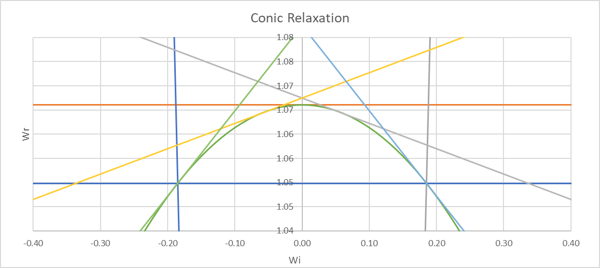
Instead of a quadratic SOCP constraint, KAIROS applies an envelope of linear segments on the apparent power where: \(W_{i} · W_{j} \ge (W^r_{ij})^2 + (W^i_{ij})^2 \)
Is represented as, where \((α)\) represents each cutting plane used to represent the quadratic envelope: \(( W_{i} + W_{j} ) / 2 \ge W^r_{ij} · cos(α) + W^i_{ij} · sin(α) \)
3.4 Meshed Networks and Linear Voltage Angle Closure
For meshed networks, KAIROS includes an envelope constraint that enforces Kirchhoff’s voltage law on voltage angles using linear constraints:
\(θ_{i}-θ_{j} \ge W^i_{ij} / cos(θ_{max,ij}/2) - tan(θ_{max,ij}/ 2) + θ_{max,ij}/ 2 - ( 1- (1-V_{max,i})^2) · sin(θ_{max,ij}) / cos(θ_{max,ij}/2) \) \(θ_{i}-θ_{j} \le W^i_{ij} / cos(θ_{max,ij}/2) + tan(θ_{max,ij}/ 2) - θ_{max,ij}/ 2 + ( 1- (1-V_{max,i})^2) · sin(θ_{max,ij}) / cos(θ_{max,ij}/2) \)
Here, is a reference value based on nominal voltage and allowable angle differences, and defines the tolerance band. This linear formulation ensures feasibility while approximating voltage consistency in loops.
Conclusion
KAIROS provides a technically robust architecture for AC power flow modeling across voltage levels. By leveraging squared voltage variables and auxiliary variables it maintains numerical tractability while accommodating real-world power system behavior. The combination of flexible linear approximations and conic envelope constraints enables KAIROS to handle both radial and meshed networks effectively, with consistent modeling across planning and operational contexts.